Where to get a heightmap for a laser-cut relief map
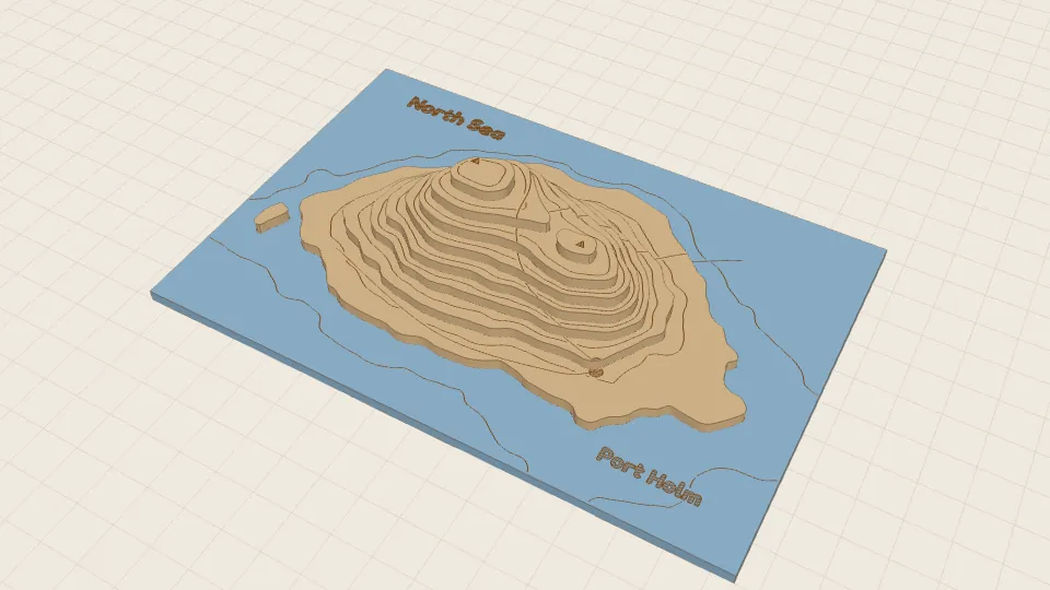
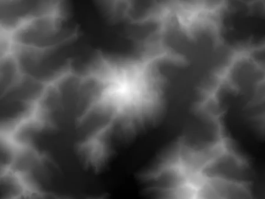
A layered relief map starts with a heightmap: a greyscale picture of the ground, light where it is high and dark where it is low. Find the right one and the rest is settings; find the wrong one and you cut a mountain with a crater on top, or a town covered in bumps. This post compares the free sources, says how much detail you actually need (less than you would think), and walks through turning elevation data into a PNG the relief map generator can read, with the checks to run before you cut.
For a complete project from heightmap to glued map, see the companion post: a laser-cut relief map of K2.
What the generator wants
- A PNG: greyscale, light = high (or tick Dark is high). Any bit depth works, 16-bit is best. Not interlaced. A colour PNG is turned into grey by brightness, so a coloured or shaded map comes out wrong.
- Square pixels on the ground, north at the top.
- Transparent pixels are off the map. Make everything outside a county, a park or a lake transparent and set Shape to outline: the map takes that shape.
- Heights are stretched between the lowest and the highest pixel, so the PNG does not need to say how high anything is. You set the real height with Relief height. That also means one bad pixel (a spike, or a hole marked as −32768) stretches everything else flat.
- Or a 3D model (STL and the like) of a terrain tile, if a tool you like exports those.
How much detail you need
The generator averages the heightmap down to at most 300 cells along the long side before it cuts it into layers. On a 200 mm map a cell is 0.67 mm, about the narrowest strip of plywood that survives cutting anyway. So the detail you need from the data is the width of your area divided by 300:
| Area across | Detail the generator keeps | Data that is fine enough |
|---|---|---|
| 300 m (a hill, a quarry, a cove) | 1 m | 1 m LiDAR |
| 3 km (a village, a lake) | 10 m | National 1-5 m data |
| 10 km and more (a mountain, a valley) | 33 m | Global 30 m data |
| 100 km (a mountain range, an island) | 330 m | Global 30 m or 90 m data |
| 1,000 km (a country, a sea) | 3.3 km | GEBCO, or 90 m data averaged down |
Finer data than that does no harm (it is averaged), but it is a bigger download for nothing. Coarser data loses the small ridges and valleys: the layers come out rounder and plainer.
Two practical consequences:
- For most mountains and islands, free global 30 m data is all you need. K2's 18 km map used 600 pixels of 30 m data and the generator kept 300 of them.
- Pick the pixel count to suit: 300, 600 or 900 pixels on the long side divide evenly into 300 cells. A 1,000-pixel image is averaged in blocks of four, to 250 cells.
8-bit or 16-bit?
An 8-bit PNG has 256 grey levels, a 16-bit one 65,536. Take Mount Fuji, framed so that the lowest point is 230 m and the summit 3,764 m: in 8 bits that is one grey level every 14 m. Shade the two files so that the slopes show, and on the gentle lower flanks the 8-bit one is all terraces:
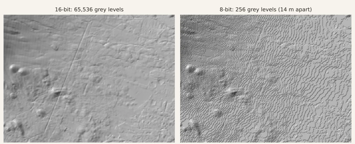
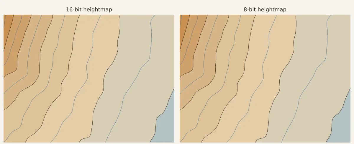
That matters for a 3D print or a CNC carving, which follow the surface. A layered map is terraces anyway: 12 sheets for those 3,500 m is one step per 295 m, about 21 grey levels per sheet. On top of that, the generator averages the pixels into its cells (3 × 3 here) and smooths them by 1 mm before it outlines a layer, which fills the 14 m steps in. Cut from the two files, the layers are the same: their edges are 0.02 mm apart on average, and 0.6 mm at the worst point.
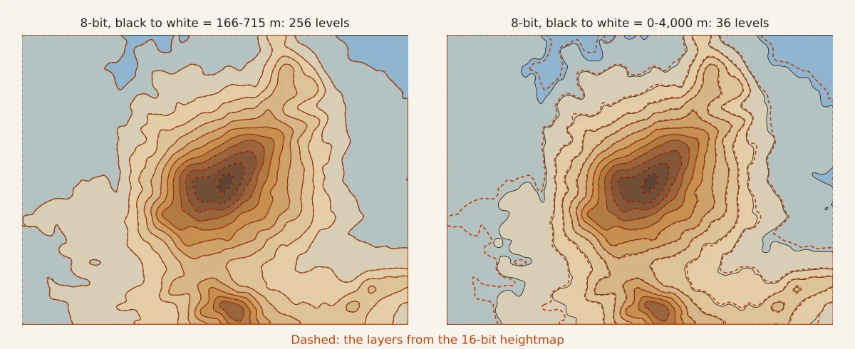
Where 8 bits do hurt is a heightmap that wastes its grey range. If black and white stand for much more than the heights in the picture (a heightmap exported with a fixed range of 0-4,000 m, or cropped from a bigger one), the map gets only a few levels. Ślęża, a lone 718 m hill on the plain south-west of Wrocław, rises 550 m above the frame's lowest point. With black at 166 m and white at 715 m, its 8-bit heightmap uses all 256 levels and the layers match the 16-bit ones. With black at 0 m and white at 4,000 m it gets 36, three per sheet, and the low layers go wrong where the ground is flattest: their edges move by 1.6 mm on average, and on the plain whole lobes of a layer appear or vanish. More Smoothing helps only a little (3 mm brings the 1.6 mm down to 1.1).
So:
- Use 16-bit when you can. From GDAL or the script below it costs nothing.
- 8-bit is fine if black is the lowest point of your map and white the highest. Check the darkest and lightest pixels in an image editor.
- Never crop an 8-bit heightmap down to a small part of it: the crop keeps only the grey levels that part had. Choose the area first, then export.
The sources
Global, about 30 m
| Source | What it is | Coverage | Surface or bare ground | Get it |
|---|---|---|---|---|
| Copernicus DEM GLO-30 | Radar (TanDEM-X), early 2010s | The whole world | Surface: includes forest and buildings | Free, no account, AWS Open Data (one GeoTIFF per 1° tile) |
| SRTM / NASADEM | Radar, February 2000 | 60° N to 56° S | Mostly surface (the radar partly sees through trees) | USGS EarthExplorer (free account), OpenTopography (free API key) |
| ALOS World 3D (AW3D30) | Optical stereo, 2006-2011 | The whole world | Surface | Free account on JAXA's site, or OpenTopography |
| FABDEM | Copernicus with forest and buildings removed (University of Bristol) | The whole world | Bare ground | Free download, non-commercial use only |
Start with Copernicus. It has no holes, and on steep ground it did best in my tries: when I made the K2 map, older data built partly on SRTM gave K2 a noisy bowl for a summit, and Copernicus a clean peak. SRTM has voids (holes) on steep slopes and in deserts; NASADEM is SRTM reprocessed with most of them filled.
Surface or bare ground matters for towns and forests, not for mountains. A surface model puts houses and tree canopy on top of the ground. On a mountain map, where one 3 mm layer stands for 100 m or more, a 25 m forest is noise. On a map of a gently rolling town, where a layer might be 10 m, the buildings become the relief. For those, use bare-ground data: FABDEM for a gift (it is non-commercial), or the national data below.
National, 1-5 m
Many mapping agencies publish LiDAR elevation for free, as bare-ground models (often called DTM) with surface models (DSM) beside them:
- United States: USGS 3DEP, 1 m where LiDAR has been flown, through The National Map download page. Public domain.
- England: the Environment Agency's LIDAR composite DTM, 1 m, free to download in 5 km tiles. Scotland and Wales have their own portals.
- Switzerland: swisstopo's swissALTI3D, 0.5 m and 2 m, open data with the source credited.
- Poland: GUGiK's NMT on geoportal.gov.pl, 1 m and 5 m, free for any use.
- Elsewhere: search for your country's mapping agency and "LiDAR DTM". Most of Europe is now open.
These come as tiles a few kilometres across, in the country's own grid (in metres, so the pixels are already square). Join the tiles you need in QGIS before exporting (step below). At 1 m they are only worth it for small areas; for anything over 10 km, the global data is as good once averaged.
The seabed and lakes
GEBCO publishes a yearly grid of the whole planet, land and seabed, at 15 arc-seconds (about 450 m at the equator). It is free to use, including commercially, with GEBCO credited, and must not be used for navigation. At 450 m it suits maps of a sea, a big lake or an ocean ridge 150 km across and up; for a small lake, look for the national lake survey. Depths come as negative heights, so the seabed is dark and the land light: tick Dark is high for a map where the deepest point is the tallest layer, and raise Sea level until the land (now the lowest ground) is flat.
Web map tiles
The terrain tiles behind many web maps (the Terrarium tiles on AWS, Mapbox Terrain-RGB) are easy to fetch for any place, but they are not greyscale: they pack the height into the red, green and blue values. Loaded as they are, the generator reads brightness, which is nonsense. Decode them first (Terrarium: height = R × 256 + G + B / 256 − 32768 m), stitch the tiles and save a 16-bit grey PNG. They mix several sources of different ages and quality; the Terrarium tiles credit USGS (3DEP, SRTM, GMTED2010) and NOAA (ETOPO1).
Tangram Heightmapper shows the Terrarium tiles as a grey map in the browser and saves what is on the screen: the fastest way to a heightmap, with nothing to install. The picture is 8-bit, and its auto-expose sets black and white to the lowest and highest point in view, which is exactly what 8 bits need (above). So frame the view to your map before you export, rather than cropping afterwards. Web map pixels are square on the ground (for an area up to a few tens of kilometres) and north is up. Look at the export before using it: with the render multiplier above 1 it is put together from several screens, and a part that had not finished loading can come out blank or exposed differently from the rest.
Ready-made 3D models
Tools such as TouchTerrain and Terrain2STL export a terrain tile as an STL with a base, from the same global data. The relief map generator takes those as a 3D model: it ignores the base block and uses the top surface. It is the quickest route if you already use one of them, but you give up control over the frame, the pixel size and the data source.
Turning elevation data into a PNG
Elevation data comes as GeoTIFF (or ASCII grids), in metres. Three things have to happen on the way to a PNG:
- Square pixels. Global models are in latitude and longitude, and away from the equator a degree of longitude is shorter than a degree of latitude: at 50° N, only 64 % as long. Used as is, the map is stretched sideways by more than half. Reproject to UTM (or your national grid), which is in metres. National data and web tiles already have square pixels.
- 16 bits, black at the lowest point and white at the highest (see 8-bit or 16-bit? above).
gdal_translate -scalebelow does both. - Holes filled. Voids are marked with a "no data" value (often −32768). Fill them, or they become pits at the bottom of the height range.
In QGIS (or GDAL on the command line, which QGIS installs): load the tiles, merge them (Raster > Miscellaneous > Merge), then
# reproject to UTM at 30 m and clip; xmin ymin xmax ymax in the zone's metres
gdalwarp -t_srs EPSG:32633 -tr 30 30 -r bilinear -te xmin ymin xmax ymax merged.tif area.tif
gdal_fillnodata area.tif filled.tif          # fill voids, if gdalinfo -stats shows any
gdalinfo -stats filled.tif                   # read the minimum and maximum height
gdal_translate -of PNG -ot UInt16 -scale MIN MAX 0 65535 filled.tif map.png
(EPSG:32633 is UTM zone 33 North, 12-18° E. Each zone covers 6° of longitude: zone = (longitude + 180) / 6, rounded down, plus 1; 326xx is north of the equator, 327xx south.)
With a script: the K2 post's heightmap.py makes the PNG from Copernicus (which has no
holes) for any place north of the equator: give it a centre, a width and a height in kilometres. It reads the data
straight from AWS, so there is nothing to download first. The area has to fit in one 1° tile; across a tile edge,
merge the tiles first.
pip install rasterio numpy pillow
python heightmap.py 45.83 6.86 12 9 mont-blanc.png     # centre lat, lon, width and height in km
Check it before you cut
Five checks, in a minute:
- The shape is right. Compare it with an online map: if the mountain looks too wide, the pixels are not square. If it is upside down or mirrored, north is not at the top.
- The heights are plausible. The highest pixel should be close to the published summit height. A 30 m grid usually comes out a few tens of metres short on a sharp peak, which is fine.
- No craters, speckle or stripes. A summit that looks like a bowl, or black dots, are voids. Fill them or use another source.
- No spikes. A bad value in a flat area (a mast, a glitch: a white dot) takes the top of the range and flattens everything else into the first few layers. Paint it out or clip the range.
- For towns: houses or ground? If streets show as grooves between blocks, it is a surface model. Use a bare-ground one.
Then load it into the relief map generator with no markings, and look at the 3D preview. Its ghost (the heightmap drawn over the layers) shows how closely the stack follows the data.
What you can do with the map
What you may do with the finished map depends on the data's licence. As I read the terms (check the current ones before you sell anything):
| Source | Gift | Sell the map | Credit |
|---|---|---|---|
| Copernicus GLO-30 | Yes | Yes | Pass on the Copernicus notice (the K2 post has the wording) |
| SRTM, NASADEM, USGS 3DEP | Yes | Yes | US public domain; crediting NASA / USGS is good practice |
| ALOS AW3D30 | Yes | Yes | Credit JAXA |
| FABDEM | Yes | No | Non-commercial licence |
| National data (EA, swisstopo, GUGiK...) | Yes | Usually yes | Each has its own credit line |
| GEBCO | Yes | Yes | Credit GEBCO; not for navigation |
| Terrarium web tiles | Yes | Check each source | USGS and NOAA |
A credit line engraved on the underside of the base is a nice touch and covers most of them.
Open the Relief map generator · A complete project: K2
Data credit
The Fuji and Ślęża pictures are made from Copernicus WorldDEM-30 © DLR e.V. 2010-2014 and © Airbus Defence and Space GmbH 2014-2018 provided under COPERNICUS by the European Union and ESA; all rights reserved. The organisations in charge of the Copernicus programme by law or by delegation do not incur any liability for any use of the Copernicus WorldDEM-30. laserpuzzle is not endorsed by the European Commission, ESA, DLR or Airbus.